Abstract
Cristian Ramírez · Literature checked: 22 November 2026.
Matrix multiplication has two different optimization frontiers. Algebraic complexity asks how the number of exact arithmetic operations grows with dimension. Performance engineering asks how a particular implementation uses finite registers, memory, arithmetic units and energy. Their interaction is productive precisely because the answers are different. Seven block products can replace eight, yet a carefully packed cubic kernel can outperform a more sophisticated construction at the sizes a machine can hold.
This article develops the bridge between those frontiers. It derives Strassen’s identity and recurrence, introduces tensors, restrictions, border rank and the asymptotic sum inequality, and follows fifteen historical milestones from 1969 to the 2024/2025 asymmetric laser method. It then examines research released in 2026, distinguishing an optimization certificate, available formal proof artifacts, independent follow-up manuscripts and peer review. Finally, it connects arithmetic reductions to stability, communication, BLIS-style organization and my work on integer GEMM for the RISC-V GAP8 processor.
The numerical bounds are upper bounds on a mathematical exponent, not measured speedups. Imported results are cited; short examples and cost models are derived here. I have not rerun the historical optimizers, the recent numerical certificate or the complete Lean proof closure. Some early original proofs were inaccessible; their sections identify exactly what the available primary records establish. This is a critical literature synthesis and engineering exposition, not a claim to have independently verified every proof or discovered a new exponent.
Why this problem remains open
For two dense square matrices, the familiar formula contains n³ scalar multiplications. That count belongs to one algorithm. It is not a lower bound on every possible way to compute the same bilinear map. Reusing algebraic combinations across outputs creates the possibility of doing less multiplication, while generating extra additions and more complicated data dependencies.
The gap between a quadratic output and a cubic textbook algorithm is therefore a question about representation. How economically can one express all output coefficients simultaneously? Once an economical expression exists, can its products be arranged into large independent matrix multiplications? Can a finite construction be amplified without losing its savings to interference, approximation overhead or communication? Each historical phase below changes one of those questions.
The problem also exposes the limits of a single metric. Reducing a power of n is decisive asymptotically, but does not determine coefficient growth, working memory, precision, parallelism or attainable arithmetic throughput. The engineer must inspect the algorithmic graph and the machine together. A paper that improves ω and a kernel that improves inference latency can both be important without solving the same optimization problem.
The timeline in my thesis
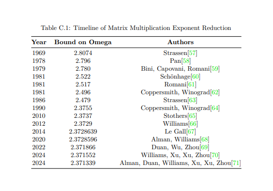
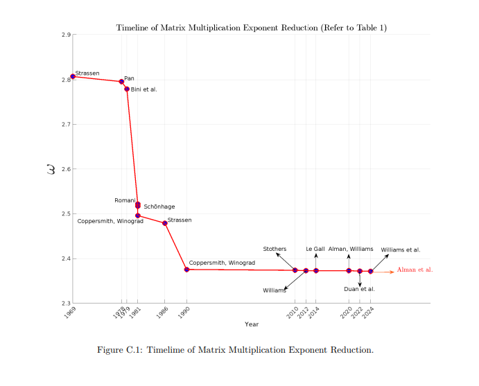
The following images reproduce the original Table C.1 and Figure C.1 from my doctoral thesis. They preserve the historical timeline as it appeared there. The image bytes are unchanged. The verified chronology below adds publication/version distinctions and research after the timeline’s endpoint; it does not silently edit the originals. Thesis attribution is given in 33.
Accessible transcription of original Table C.1
| Year | Bound on omega | Authors as displayed |
|---|---|---|
| 1969 | 2.8074 | Strassen |
| 1978 | 2.796 | Pan |
| 1979 | 2.780 | Bini, Capovani, Romani |
| 1981 | 2.522 | Schönhage |
| 1981 | 2.517 | Romani |
| 1981 | 2.496 | Coppersmith, Winograd |
| 1986 | 2.479 | Strassen |
| 1990 | 2.3755 | Coppersmith, Winograd |
| 2010 | 2.3737 | Stothers |
| 2012 | 2.3729 | Williams |
| 2014 | 2.3728639 | Le Gall |
| 2020 | 2.3728596 | Alman, Williams |
| 2022 | 2.371866 | Duan, Wu, Zhou |
| 2024 | 2.371552 | Williams, Xu, Xu, Zhou |
| 2024 | 2.371339 | Alman, Duan, Williams, Xu, Xu, Zhou |
Several entries need context. The 1979 paper also includes Grazia Lotti. Some years identify an announcement rather than the journal publication. Some numbers are conservative rounding; another combines an initial submission year with a later improved version. A plotted point also does not identify whether the inequality is strict, which field is allowed or whether a corrected manuscript supersedes an earlier headline. Those distinctions belong in the textual analysis, not in a fabricated replacement figure.
Classical multiplication and the arithmetic model
Let F be a field, with A in F to the m-by-k power and B in F to the k-by-n power. The exact product is defined by
For square order n, independent dot products require n³ multiplications and n²(n−1) additions when a length-n sum starts from its first term. The total is 2n³−n². An implementation that instead accumulates into an existing C can execute n³ additions. The usual leading count 2n³ treats a multiply-add as two floating-point operations even when one FMA instruction executes it. Arithmetic operations, instructions and cycles are different counts.
Loop interchange, packing and cache blocking can radically change runtime while preserving these classical operation counts. Conversely, an algebraic algorithm can reduce multiplication count while adding data movement. The distinction prevents a common mistaken inference: observing a faster blocked implementation is not evidence that it has a smaller exponent.
Define the square arithmetic exponent over F by
Here MM counts exact field additions, subtractions and multiplications in the specified arithmetic model. Constants may depend on the fixed field and algorithm; the dimension is the asymptotic variable. In this article, finite bilinear identities and their division-free recursive evaluation are the main model. Reading input, writing output, finite-word arithmetic and memory transfers require additional accounting on a machine. The conventional range is 2 ≤ ω ≤ 3; the lower endpoint is a basic dimensional obstruction, not evidence that quadratic multiplication has been constructed.
The infimum and positive slack matter. A theorem ω ≤ τ generally provides, for every ε > 0, an O(n to the τ+ε) family. It need not give one uniform O(n to the τ) routine with a modest constant. The base algorithm may depend on ε, and become enormous as ε decreases. Replacing that quantifier structure with a short executable kernel would materially change the claim.
Fields, bits and rectangular shapes
One exact addition in Q is not one constant-time machine instruction. Rational numerators and denominators grow; integer multiplication depends on bit length. Floating-point operations obey a different, rounded semantics. An arithmetic exponent can inform bit-complexity analysis, but does not supply it without coefficient-size and precision bounds.
Field extensions also need accounting. A fixed extension of degree d can be represented in a fixed basis and simulated using a bounded number of base-field operations depending on d. Thus a fixed complex operation can be simulated by a constant number of real operations on two coordinates, and real identities extend to complex inputs. This gives equality of the corresponding real and complex arithmetic exponents in this model. It does not equate their hardware cost or stability.
A complex constant need not be rational, so the same two-coordinate argument does not descend to Q. Algebraization or number-field descent needs its own proof. Extensions whose degrees grow with n are another case: polynomial growth can alter the exponent, while polylogarithmic degree with polynomial simulation cost contributes only subpolynomial overhead. Fixing ε, then fixing a finite construction and its coefficient field, then letting n grow is different from enlarging the field with every input dimension.
Finally, write ω(a,b,c) for the exponent of multiplying an nᵃ-by-nᵇ matrix by an nᵇ-by-nᶜ matrix. The square case is ω(1,1,1). The dual exponent α is conventionally the supremum of k for which ω(1,k,1)=2. A new rectangular or dual bound can be significant without being the same number as a square bound. Shape is also a central practical variable: a long reduction dimension and two small outer dimensions expose different reuse and parallelism from a square product.
Bilinear maps, tensors and asymptotic extraction
An exact bilinear algorithm computes products of linear forms in the two inputs and linearly recombines them. If entries of A and B are indexed by single coordinates a and b, an r-product algorithm has the form
The coefficients are fixed elements of F, independent of the inputs. They express a reusable identity, not products chosen after seeing particular zeros. Encoding the output with dual variables gives the trilinear form
The z indices close the cycle. The z variables record outputs; evaluating this form is a way to encode all coefficient identities simultaneously. Permuting the three tensor legs relates different rectangular products, but does not license exchanging the order of noncommuting matrix factors inside an implementation.
The tensor rank R(T) is the least number of simple tensors whose sum is T. A rank-r decomposition supplies r bilinear products. Additions and scalar linear maps still cost work. For a fixed base construction used recursively, their quadratic work per node can be absorbed in the resulting subcubic arithmetic recurrence. If the base construction itself grows with the input, that argument must be revisited.
Tensor products encode simultaneous independent choices at each recursive level:
A restriction applies linear maps separately to the three legs. Zeroing selected variables is an especially transparent restriction. A degeneration permits parameter-dependent maps whose leading coefficient or limiting form is the target. Write S ⊑ T for a degeneration from T to S. The direction matters: an economical source can produce a target, not conversely.
Border rank: a limit of exact expressions
The border rank, written below with an underline, is the smallest r for which T is a degeneration of r simple products. It can be lower than exact rank. Approximation here is algebraic: a parameter tends to zero, and the desired tensor appears as a specified coefficient. It is not a guarantee that substituting a tiny floating-point number gives an accurate computation.
An independently derived example makes the distinction concrete. In two-dimensional spaces with basis e₀,e₁, set
Expanding the following expression yields W plus terms divisible by t:
For nonzero t the left side is a sum of two simple tensors, with scalar factors absorbed in a leg. Therefore its border rank is at most two. A leg flattening has rank two, so the border rank is exactly two. The displayed expansion alone does not prove an exact rank-two decomposition of W; it only proves a degeneration. This example is not a claimed historical construction for matrix multiplication.
To turn a degeneration into exact asymptotic arithmetic, one can extract coefficients by interpolation after taking tensor powers. If one fixed degeneration has degree d, its Nth power has degree at most dN. Over a sufficiently large field, recovering a coefficient costs only O(dN) evaluations, a factor whose Nth root tends to one. Small finite fields require extension and descent accounting. This is the mechanism behind why border rank can control an exact arithmetic exponent; it is not an instruction to divide by an infinitesimal on a processor. Bini’s later exact/approximate conversion supplies the historical bridge 5.
The asymptotic sum inequality
Suppose a tensor with border rank at most r degenerates to a direct sum of matrix products, with disjoint variable spaces in all three legs. The asymptotic sum inequality gives
Field hypotheses and coefficient extraction accompany this asymptotic statement; it is not an equality of finite ranks. A shared variable can spoil direct-sum independence even when two displayed products look separate. Much of the laser method is devoted to extracting enough products while eliminating precisely those unwanted interactions 6, 10.
For an illustrative check, two independent 2-by-2 products can each use Strassen’s seven products, so their direct sum has rank at most fourteen. The inequality becomes
This intentionally recovers the existing bound. It creates no improvement merely by writing a direct sum. An improvement needs a source that packs the independent products more economically than paying separately for them. That is the conceptual step beyond a single block recurrence.
1969 — Strassen: seven products replace eight
Volker Strassen’s Gaussian Elimination is not Optimal establishes a finite exact identity, the most direct possible challenge to the cubic intuition 1. Partition A and B into four equally sized square blocks. The seven products are
Recombine them as
For example, expanding the first output gives
Every unwanted cross term cancels. The operand order is preserved, so the identity works for matrix blocks and, more generally, over a ring with subtraction; it does not rely on commuting A and B blocks. The other three outputs expand in the same explicit way. Multiplication uses no division, unlike an inversion procedure whose pivots may impose additional assumptions.
There are ten block additions/subtractions to prepare operands and eight to recombine results. With square order a power of two and a fixed leaf threshold,
The recurrence counts arithmetic with unit-cost entries. Its exponent comes from the seven children, while the quadratic additions give a lower-order contribution. A finite rank identity has become an asymptotic algorithm. This is a constructive upper bound, not a matching lower bound on all multiplication methods.
For arbitrary positive n, pad to the next power of two p. Since n ≤ p < 2n, the asymptotic exponent is unchanged, but the constant and wasted work can be substantial. A real library can instead peel irregular edges or choose shape-aware recursion. Mathematical padding is a correctness argument; it is not necessarily an implementation recommendation.
A tested executable identity
The following standard-library Python source is shared by both language versions. It accepts equally sized square matrices, recursively pads and crops, and uses a configurable classical leaf. Integers and Fraction support exact arithmetic; using floats changes the numerical semantics. This allocating implementation is pedagogical, with no claim of BLAS-level performance or an experimentally tuned cutoff.
"""Educational square-matrix multiplication over an exact ring.

Use immutable entries supporting +, -, *, and integer zero, such as int or
fractions.Fraction. No floating-point conversion or input mutation is performed.
These allocating Python routines demonstrate identities, not optimized BLAS.
"""


def _validate(a, b):
    for matrix in (a, b):
        if not isinstance(matrix, (list, tuple)):
            raise TypeError("matrices must be lists or tuples of rows")
        if any(not isinstance(row, (list, tuple)) for row in matrix):
            raise TypeError("matrix rows must be lists or tuples")
        if any(len(row) != len(matrix) for row in matrix):
            raise ValueError("each matrix must be square")
    if len(a) != len(b):
        raise ValueError("matrices must have the same order")
    return len(a)


def _classical(a, b):
    n = len(a)
    c = [[0] * n for _ in range(n)]
    for i in range(n):
        for k in range(n):
            for j in range(n):
                c[i][j] += a[i][k] * b[k][j]
    return c


def classical(a, b):
    """Return a*b for equally sized square matrices; [] represents order zero."""
    _validate(a, b)
    return _classical(a, b)


def _combine(a, b, subtract=False):
    return [[x - y if subtract else x + y for x, y in zip(ar, br)]
            for ar, br in zip(a, b)]


def _split(a):
    h = len(a) // 2
    return ([row[:h] for row in a[:h]], [row[h:] for row in a[:h]],
            [row[:h] for row in a[h:]], [row[h:] for row in a[h:]])


def strassen(a, b, leaf_size=32):
    """Return a*b with seven-product recursion and classical leaf products.

    Pad to p, the next power of two, and crop the returned matrix to order n.
    leaf_size must be a positive int (bool is rejected); it is a teaching
    parameter, not a measured crossover. Entries are not type-restricted:
    exactness requires exact ring operations; floats do not gain that property.
    """
    if type(leaf_size) is not int:
        raise TypeError("leaf_size must be an integer")
    if leaf_size < 1:
        raise ValueError("leaf_size must be positive")
    n = _validate(a, b)
    if n == 0:
        return []
    p = 1 << (n - 1).bit_length()

    def pad(matrix):
        return ([list(row) + [0] * (p - n) for row in matrix]
                + [[0] * p for _ in range(p - n)])

    def multiply(x, y):
        if len(x) <= leaf_size:
            return _classical(x, y)
        a11, a12, a21, a22 = _split(x)
        b11, b12, b21, b22 = _split(y)
        add = _combine

        def sub(u, v):
            return _combine(u, v, subtract=True)

        m1 = multiply(add(a11, a22), add(b11, b22))
        m2 = multiply(add(a21, a22), b11)
        m3 = multiply(a11, sub(b12, b22))
        m4 = multiply(a22, sub(b21, b11))
        m5 = multiply(add(a11, a12), b22)
        m6 = multiply(sub(a21, a11), add(b11, b12))
        m7 = multiply(sub(a12, a22), add(b21, b22))
        c11 = add(sub(add(m1, m4), m5), m7)
        c12 = add(m3, m5)
        c21 = add(m2, m4)
        c22 = add(add(sub(m1, m2), m3), m6)
        return ([u + v for u, v in zip(c11, c12)]
                + [u + v for u, v in zip(c21, c22)])

    product = multiply(pad(a), pad(b))
    return [row[:n] for row in product[:n]]
From the repository root, run python -B examples/matrix-history/test_strassen.py. The thirteen tests check the identity with formal noncommuting polynomials, multiplication counts, exact random integers and fractions, odd dimensions, padding, invalid inputs and input preservation. Exact tests validate these algebraic identities and cases; they do not establish a floating-point error bound.
With depth-first evaluation, peak auxiliary storage is O(p²) matrix-entry slots and recursion depth O(log p). This counts live slots, not cumulative allocation or bits inside growing exact numbers. The seven intermediates still occupy memory, and Python object overhead is outside the arithmetic model. Both the algorithm and its stated limitations are part of the example.
1978 — Pan: aggregation changes the unit of optimization
Victor Pan’s trilinear aggregation moved beyond recursively repeating a tiny square identity. The target becomes a collection of products represented together, so that useful terms can share an aggregate expression and unwanted terms are explicitly canceled. The 1978 FOCS work is the historical milestone; Pan’s later original journal paper documents the aggregation, uniting and cancellation approach 2, 3.
A small schematic expansion explains the attraction and the difficulty. For independent symbols, an aggregate gives
Two desired trilinear terms appear in one aggregate, but so do six interference terms. This is not Pan’s algorithm or a rank improvement: paying for each correction separately could erase all savings. A successful construction arranges many such expressions so that the corrections themselves have an economical structure. Counting only the desired diagonal terms would be an invalid complexity analysis.
The 1979 Bini paper reports Pan’s bound at approximately 2.7951, supporting the conservative timeline entry 2.796. I did not obtain a readable original 1978 proof, and therefore do not claim to reproduce its exact aggregation parameters or field restrictions. In particular, a commonly quoted large base decomposition is not promoted here to a checked theorem merely because its logarithm numerically matches the bound.
The conceptual significance is nevertheless clear: the optimization space now includes combinations of products rather than one local recurrence. The engineering consequence is a question, not an automatic speedup. How many temporary linear combinations and correction passes does the construction need, and can they share packing or stay in fast memory? Without that mapping, an arithmetic saving may increase traffic. Aggregation introduces algebraic reuse that must later be converted into physical reuse.
1979 — Bini, Capovani, Romani and Lotti: approaching a tensor
The two-page original by Dario Bini, Milvio Capovani, Francesco Romani and Grazia Lotti studies approximate bilinear constructions with a parameter tending to zero 4. The missing fourth author in the thesis image must be restored in the scholarly account. The resulting square construction has the arithmetic count summarized by
The paper combines rectangular approximate products and cyclic variants to obtain this dimension/product-count relationship. The approximation parameter belongs to an algebraic limiting argument. The separate 1980 Bini paper supplies the exact-versus-approximate interpolation relation 5. It would be historically and mathematically inaccurate to treat a fixed-precision substitution in the 1979 formula as that exact conversion theorem.
Why can a limiting construction help an exact exponent? Fix a degree-d degeneration before amplification. An Nth tensor power has at most linearly growing degree dN, while the useful product count grows exponentially in N. Coefficient extraction adds a polynomial factor in N; taking Nth roots removes it in the asymptotic comparison. The gain comes from the ordering of those limits, not from ignoring approximation error.
For numerical computation the situation reverses: expressions divided by a small parameter can magnify rounding and cancellation. Choosing a smaller parameter reduces truncation error but may increase roundoff or coefficient range. The exact-arithmetic interpolation argument bypasses that numerical procedure; it does not prove that the naive limiting evaluation is stable. The original letter itself leaves practical bit cost and stability unresolved.
This milestone broadens the search from decompositions that equal the tensor at every parameter value to families that approach it. Border rank becomes an algebraic resource. The essential discipline is to keep three claims separate: an approximate identity, an exact asymptotic conversion, and a stable finite-precision implementation. None follows from writing the other two words beside a decimal exponent.
1981 — Schönhage: independent products have collective value
Arnold Schönhage’s Partial and Total Matrix Multiplication links approximate rank and simultaneous products 6. Its publisher record states an arbitrary-field bound slightly below
The asymptotic sum inequality is the structural development that outlives the particular decimal. Its formulation is reconstructed in the original CW1990 paper, which was readable even though Schönhage’s full proof was not available in this audit 10. If a source of approximate rank L yields disjoint products, solve the monotone equation
The resulting arithmetic exponent is at most 3τ, with positive exponent slack in a concrete runtime statement. The factor three converts volume of a product tensor into square dimension. Omitting it would confuse tensor volume with matrix order.
For example, suppose a hypothetical source gave two independent products with volumes v₁ and v₂. Its feasibility inequality would compare L with v₁ to the τ plus v₂ to the τ, not with the larger volume alone. Both outputs contribute. Conversely, merely placing them in a shared algebraic expression does not establish independence: every input and output leg must split appropriately. A partial product can be valuable because later amplification and extraction use its structure, rather than because it is already a full square multiplication.
This reframes the design objective as the productive content of a source tensor. It helps explain why later constructions often look remote from executable GEMM. They first create many potential products, then isolate a useful direct sum, then invoke an asymptotic theorem. The sequence proves existence of an arithmetic algorithm; it still leaves an implementation problem involving sizes, coefficients, extraction and memory organization.
1981/1982 — Romani: the analysis of disjoint sums
Francesco Romani’s Some Properties of Disjoint Sums of Tensors Related to Matrix Multiplication appeared in the journal in May 1982 7. The thesis places the milestone at 1981 and prints 2.517. The publisher abstract confirms an approach through ranks of powers of a disjoint sum and a transcendental equation, but does not expose the full equation. The original scan could not be read here. Accordingly, 2.517 remains a historical figure entry whose exact construction is not independently reconstructed in this article.
The mathematical issue can still be explained without inventing Romani’s proof. If S and T represent independent tasks, then
This is a general distributive identity, not the inaccessible paper’s claimed optimized equation. Tensor positions encode the choice of S or T. There are binomially many words with each frequency, and a product dimension depends exponentially on that frequency. When N grows, a balance between multiplicity and product size emerges. An equation involving exponential functions of the exponent is natural because both resources are exponential before the Nth root is taken.
The independent lesson is that one cannot optimize a direct sum by examining each summand in isolation. The powers contain mixed types. A particular choice of frequency can change the asymptotic extraction bound, and boundary frequencies can behave differently from balanced ones. Later entropy formulations make that balance explicit.
For engineering, these binomial multiplicities are also a warning. A proof can select one useful asymptotic type while discarding large regions of an intermediate construction. The count of useful arithmetic products says little about the storage or setup cost of literally materializing that construction. The section therefore preserves the milestone while clearly locating its evidence gap, rather than attaching a generic tensor-power equation to Romani as if it were his verified theorem.
1981/1982 — Coppersmith and Winograd: below 2.5
Don Coppersmith and Shmuel Winograd’s early On the Asymptotic Complexity of Matrix Multiplication has a 1981 FOCS version and a 1982 journal publication 8. The original publisher abstract states ω < 2.495548, a more precise version of the thesis’s 2.496. It also discusses acceleration. The complete early proof and its detailed field hypotheses were not readable in this audit; the bound is cited at that evidence level.
Crossing 2.5 matters historically because the reduction is no longer a small refinement of seven-versus-eight multiplication. The previous tools—aggregation, limiting rank and simultaneous products—have changed what counts as a usable starting point. A finite source need not be a small square multiplication with a transparent recursive schedule.
One can quantify what a local base construction would imply without claiming to reproduce theirs. If an order-b identity has r products and fixed quadratic preparation, then
Thus r < b to the 5/2 would cross 2.5 in that model. An acceleration or asymptotic extraction theorem can establish a bound without presenting exactly this small finite identity. Confusing these two routes obscures where constants and limiting arguments enter.
Likewise, a limitation proved for a specified acceleration framework is not an unconditional lower bound on ω. A theorem about a fixed base, restricted tensor family or selected extraction procedure cannot exclude algorithms outside that class. This distinction becomes essential when interpreting later laser-method barriers. A method may be unable to reach two even while the true exponent remains unknown.
The practical consequence is not that every sub-2.5 construction is unusable by definition. It is that its implementation cannot be judged from the exponent alone. A reviewer needs an explicit finite algorithm, coefficient control, shape restrictions and a schedule before any runtime or numerical claim can be evaluated.
1986 — Strassen: the laser viewpoint
Strassen’s later work introduces a tensor-based extraction viewpoint rather than another version of his seven-product identity 9. The conference work must be distinguished from the related 1987 and 1988 journal developments. The readable CW1990 reconstruction gives, for the relevant construction,
At q=5 this yields
These formulas are sourced to the original CW reconstruction, not represented as an independent reading of the inaccessible 1986 proof 10. The denominator four records the simultaneous productive content of the construction. Dropping it loses the gain; treating it as four free copies without verifying extraction would invent one.
The laser metaphor refers to retaining selected components of large tensor powers while zeroing incompatible variables. A tensor is partitioned into blocks. Tensor powers create sequences of blocks. By choosing frequencies and enforcing compatibility, one extracts a direct sum whose summands have matrix-multiplication structure. The source’s low border rank pays for all of them together.
This is a shift from the local question “how many products form one small matrix multiplication?” to “how much multiplication can be isolated from a structured source?” The selected products can be rectangular and become square only after cyclic combination. Volume, multiplicity and symmetry now interact. The next section’s progression-free sets are a way to prevent the collisions that otherwise couple those selected products.
The engineering distance from a finite microkernel grows accordingly. A tensor component may be useful because of what its very high powers contain, not because the component by itself is a desirable operation on a CPU. Nevertheless, the reasoning introduces an enduring performance-analysis habit: distinguish productive work from interference, and account for the cost of isolating the productive part.
1990 — Coppersmith–Winograd: arithmetic progressions and structured powers
Matrix Multiplication via Arithmetic Progressions combines a low-border-rank tensor with combinatorial extraction 10. The journal appeared in 1990; earlier report and conference versions explain dates in the late 1980s. Its abstract rounds to 2.376, while §8 gives ω < 2.375477. The thesis’s 2.3755 is conservative rounding, not a competing theorem.
For q positive, the familiar CW form can be written
Group each leg into levels 0,1,2: coordinate 0; coordinates 1 through q; coordinate q+1. Nonzero components have level indices summing to two. This tight support persists through tensor powers, where coordinatewise level sums organize the components. The compact border rank and rich support coexist; the extraction analysis exploits both.
Why arithmetic progressions? A hashing scheme assigns labels related by a linear relation. Restricting labels to a set without nontrivial three-term progressions helps force surviving matches to have the intended common label. One must also prune collisions and shared variables. A progression-free condition alone is not a complete direct-sum proof, but it supplies a way to keep many compatible choices without retaining unwanted triples.
For a word of N component choices with frequencies P(s), the number of such words is a multinomial coefficient:
for fixed finite support S and integral frequencies. The logarithmic remainder depends on that fixed support. Entropy measures exponential multiplicity. It does not measure hardware disorder or bytes transferred. Surviving product dimensions and the source rank are also exponential in N, so taking logarithms produces an optimization problem over distributions.
The durable achievement is the source tensor plus a framework for analyzing its powers. Later reductions often retain the source and improve how much value can be extracted. The journal’s discussion already warns about impractical parameters; it supplies no modern crossover measurement. The twenty-year plateau after this work is a plateau in the known upper bound, not evidence that practical GEMM engineering stopped improving.
2010 — Stothers: fourth powers and compatible distributions
Andrew James Stothers’s Edinburgh thesis analyzes higher powers of the CW construction 11. Its fourth-power analysis improves the longstanding bound. The later joint paper with A. M. Davie gives ω < 2.373689703 and attributes the improvement to the 2010 work 12. The thesis’s 2.3737 is a conservative historical summary. The thesis and journal publication are two records of one development, not two independent reductions.
Taking a fourth power is not enough by itself. A tensor product multiplies the elementary rank bound just as it multiplies available components. The gain must come from exploiting the structure of grouped components more effectively. Higher powers expose component types whose value is not captured by treating every base choice independently.
A specific issue in the Davie–Stothers analysis is a compatibility fiber: several distributions over component classes have the same three coordinate marginals. Their fourth-power organization has ten symmetry classes and a two-dimensional freedom in its marginal constraints. The paper derives weighted entropy-stationarity equations including
These b variables use that paper’s class weights; they are not arbitrary unweighted probabilities. The equations show that numerical parameters must satisfy structural constraints. Merely selecting ten attractive values does not define a valid laser construction.
An independent smaller example clarifies why marginal information can be insufficient. Consider the joint distribution
Every row and column marginal is (1/2,1/2), but
Its maximum is log 4 at x=1/4; at x=0 it is log 2, using 0 log 0=0. Equal marginals therefore do not imply equal numbers of joint words at exponential scale. This is an abstract probability illustration, not a replacement for the paper’s ten-class construction. It isolates the reason an entropy optimization over compatible joint types can matter.
The engineering analogy is limited but useful: aggregate utilization counts can hide which operands must coexist. Compatibility is an algebraic constraint here, not a cache model. The mathematical improvement comes from understanding that hidden coupling in a higher power, not from a newly measured memory schedule.
2012 — Vassilevska Williams: systematic higher-power analysis
Virginia Vassilevska Williams develops tools for automating the analysis of larger powers and their component constraints 13. The conference abstract’s 2.3727 claim was corrected. The author’s July 2014 long manuscript explicitly identifies the error and reports ω < 2.372873; its conservative eighth-power conclusion is ω < 2.3729 14. Repeating the original abstract without that correction would make the chronology misleading.
The central advance is a systematic analysis procedure. A power contains many component types. Some are immediate matrix multiplications; others need a recursive lower bound on their value. These bounds feed the next level’s constrained optimization. The task becomes a hierarchy of component analyses, not a single search for an r-product identity.
The logical direction is important. A feasible parameter vector and valid component-value lower bounds establish a sufficient inequality for an upper bound on ω. An optimizer’s inability to find a better point does not establish that the true optimum is worse, and does not establish a lower bound on ω. Constraint tolerances, normalization, zero-probability boundary cases and arithmetic precision all affect whether a computed candidate actually certifies the desired inequality.
For a generic sufficient test, let L(ρ,θ) be a rigorously justified lower bound on the productive value of a tensor power, with admissible parameters θ, and let rᴷ be its border-rank budget. Then
under the chosen value convention and extraction theorem. This displayed schema describes the proof structure; it is not a new theorem replacing the source’s constraints. The set F of feasible parameters is part of the mathematics. A point outside F, however impressive its objective value, proves nothing about the exponent.
The corrected result is also a methodological lesson. Bibliographic precision includes manuscript versions, not just author and year. The thesis’s rounded 2.3729 avoids preserving the erroneous headline, while the detailed analysis should tell the reader why the available source records disagree. Software-assisted mathematical search needs versioned inputs and auditable output just as performance experiments need versioned kernels and configurations.
2014 — Le Gall: value, entropy gaps and convex subproblems
François Le Gall’s Powers of Tensors and Fast Matrix Multiplication provides a general optimization method and reaches ω < 2.3728639 15. Its combined analysis uses powers through 32. The small decimal change hides an important algorithmic contribution: part of the analysis can be organized as convex optimization, rather than relying solely on an uncontrolled nonconvex numerical search.
To make the statement precise, use Le Gall’s value convention. Let Tᶜ and Tᶜᶜ be cyclic permutations of the legs. For 2 ≤ ρ ≤ 3, define the asymptotic value from extractions
The maximum ranges over the allowed extractions; the asymptotic definition is the source’s. Cyclic symmetrization and the factor three keep ρ in square-exponent units. Some later literature calls its parameter ρ/3 instead. Values cannot be compared across those conventions without conversion.
For a tight-support decomposition with components Tₛ and a distribution P on support S, Theorem 4.1 gives
where P₁,P₂,P₃ are the coordinate marginals and
Use one consistent logarithm base; this article uses natural logs. Tight support means that component indices lie on a fixed coordinate-sum plane in the stated decomposition. These hypotheses matter. The formula is not an entropy bound for arbitrary unrelated partitions.
The first three marginal entropies represent the available coordinate words. The component values account for productive work inside a retained block. The nonnegative entropy gap charges the ambiguity among joint types with those marginals. In the preceding two-by-two illustration, that gap would be log 4−H(Pₓ); it vanishes only at the maximum-entropy compatible coupling. The illustration explains the penalty but does not itself satisfy every tensor hypothesis of the theorem.
Le Gall’s Algorithm A first optimizes a concave expression and then chooses a maximum-entropy distribution in the fixed-marginal fiber. This gives a certified lower bound, not a global solution of every nonconvex formulation. The paper also uses a separate Algorithm B to sharpen the eighth-power analysis, then extends to powers 16 and 32. The complete story is more specific than “convex optimization solved matrix multiplication.”
For q=5, the rank budget at power 32 is 7³². Table 5 reports a positive lower-bound surplus at ρ=2.3728639. Its displayed negative lower estimate at a slightly smaller ρ is not proof that no stronger feasible construction exists. A lower estimate that misses a threshold can be inconclusive. This distinction between sufficient certificate and failed search will remain central in the 2026 optimization papers.
2020/2021 — Alman and Vassilevska Williams: refined extraction
Josh Alman and Virginia Vassilevska Williams’s A Refined Laser Method and Faster Matrix Multiplication was announced in 2020, published at SODA 2021, and later appeared in TheoretiCS in 2024 16. It establishes ω < 2.3728596 with algorithms over any field. Those dates describe versions of one development.
The refinement improves the guarantee for extracting usable disjoint components from a partitioned tensor. It does not replace the CW source with a newly found small dense GEMM kernel. Its final application studies the 32nd power of CW₅ and establishes the required value-versus-rank surplus. In the square-exponent normalization used above, the decisive comparison is
The source writes the value parameter divided by three in its own convention. The conversion here is deliberate. Quoting its value symbol with this article’s exponent convention but leaving the parameter unchanged would create a factor-of-three error.
Why can a refinement beat an earlier analysis on the same power? A source tensor’s rank budget is unchanged, but the provable amount of simultaneously extractable work can increase. Earlier bounds may discard too many candidate components to enforce independence. Better combinatorial accounting can reduce that loss without changing the algebraic source. The resulting decimal reflects a stronger lower bound on value, not a reduction in the tensor’s already known border rank.
At this stage, mathematical optimization has several layers: choose distributions, bound component values, account for collisions, and compare with the source budget. A heuristic can help find parameters, but the extraction theorem determines what those parameters mean. The distinction also explains why a very small improvement may require a substantive new proof rather than simply more optimizer iterations.
The engineering implication is indirect. The proof improves the existence theory of exact multiplication. It does not specify a practical crossover, a numerical error constant or a GPU execution schedule. Those require a finite construction and measurements with explicitly stated precision and shape. The contribution should be valued on its own mathematical terms before drawing systems conclusions.
2022/2023 — Duan, Wu and Zhou: asymmetric hashing
Ran Duan, Hongxun Wu and Renfei Zhou’s Faster Matrix Multiplication via Asymmetric Hashing changes how extraction handles combination loss 17. The first submission is from 2022; the inspected early revisions state 2.37188. The improved ω < 2.371866 appears in the April 2023 revision and the FOCS 2023 record. That is why a 2022 point with the later digits needs a version note.
Combination loss arises when individually useful components are merged at a higher level but their internal choices cannot all be retained together. Counting each component’s best possible value independently can overstate the compatible total. Conversely, enforcing a uniform symmetric treatment can discard valid combinations. The paper uses asymmetric hashing to recover value that earlier accounting loses, with its reported construction using an eighth power.
A generic count illustrates the issue without reproducing the paper’s construction. Suppose M candidate subproblems are available locally, but compatibility retains only K after a global consistency condition. The useful multiplicity is K, not M. If M and K grow exponentially with tensor power N, their ratio contributes a nonvanishing entropy-rate penalty:
If that expression tends to a positive constant, it survives the asymptotic limit. A constant-factor pruning loss, by contrast, disappears after division by N. This distinction is why correcting a combinatorial loss can improve an exponent, whereas saving a fixed number of setup operations cannot.
The paper also discusses a roughly 2.3725 barrier for a restricted earlier method. Such a barrier is not a lower bound on ω. It says that a particular analysis or extraction framework cannot certify beyond its limit under its hypotheses. The asymmetric construction changes the framework, so surpassing that barrier is consistent with the barrier theorem.
For an engineer, the lesson is about accounting: a local optimum cannot always be composed into a global optimum. This is not a claim that hashing is the missing optimization in a GEMM kernel. Here the hash functions enforce algebraic independence across tensor words; they are not an instruction to hash matrices at runtime to gain the reported asymptotic speed.
2024 — Vassilevska Williams, Xu, Xu and Zhou: complete split distributions
Virginia Vassilevska Williams, Yinzhan Xu, Zixuan Xu and Renfei Zhou’s New Bounds for Matrix Multiplication: from Alpha to Omega appears at SODA 2024, following a 2023 preprint 18. Its square theorem states ω ≤ 2.371552. The non-strict inequality is preserved here. The paper also improves rectangular bounds and gives α ≥ 0.321334; those are distinct claims.
The analysis retains complete split distributions, recording information down to level-one blocks rather than only one recursion step. A coarse marginal can hide multiple ways to realize a higher-level component. Remembering the complete lower-level split can prevent an analysis from treating incompatible realizations as interchangeable.
The additional information has a cost. All three tensor legs must satisfy consistency conditions, and some variables are missing after restrictions—described as holes in the construction. A successful extraction must repair or account for those holes. More constraints do not automatically improve an objective; they can reveal an earlier overcount. The gain comes from organizing the construction so the stronger bookkeeping remains productive.
In a schematic hierarchical distribution, let s be a coarse component and u its internal split. The joint law is
This standard identity illustrates the information discarded by keeping only P(s). It is not the paper’s complete feasibility system. The conditional distributions must also agree with the leg partitions and recursive tensor structure. Treating them as unconstrained independent variables would manufacture an unjustified entropy bonus.
The rectangular results reinforce an important distinction between theoretical and practical shape. Theory characterizes how dimensions scale as powers of n, while libraries optimize finite triples (m,k,n). Both need shape information, but an improvement in α does not predict the latency of one fixed attention matrix. A systems claim still needs dtype, layout, batch size, hardware and a measured execution path.
2024/2025 — Alman and collaborators: more asymmetry
Josh Alman, Ran Duan, Virginia Vassilevska Williams, Yinzhan Xu, Zixuan Xu and Renfei Zhou’s More Asymmetry Yields Faster Matrix Multiplication was announced in 2024 and published at SODA 2025 19. Its historical result is ω < 2.371339. A later 2026 revision incorporates a newer optimization, so an unversioned current abstract cannot establish which digits belong to 2024.
The construction relaxes a previous requirement to treat two dimensions identically in the analysis. This enlarges the admissible design space while preserving the global requirements needed to recover square matrix multiplication. It does not mean that symmetry disappears everywhere or that the final square product becomes rectangular.
A constrained-optimization analogy clarifies the logical gain. If Fsym is the subset of feasible parameter choices satisfying an added symmetry condition, then
This inclusion alone does not prove a strict improvement: a better feasible construction must still be supplied. Nor may one drop compatibility constraints simply to enlarge the search domain. The meaningful freedom is freedom justified by the tensor construction, followed by the required balancing of the three roles.
The historical sequence now has a clear structure. Higher powers exposed more component types; refined extraction reduced losses; asymmetric hashing changed compatibility accounting; complete split distributions retained more internal structure; further asymmetry removed an unnecessary restriction. These are distinct mathematical advances even when the printed exponents differ only in later decimals.
For implementation, the enlarged parameter space does not automatically yield a manageable kernel. The source, recursive decomposition and extraction remain asymptotic objects. Its relevance to performance engineering is a demonstration of careful constraint modeling and verification, rather than a benchmark result for a processor or an inference workload.
Beyond the thesis timeline: research released in 2026
The following results were inspected as of 22 November 2026. They are separated from the preceding conference/journal chronology because evidence and publication status differ. Primary manuscripts establish what their authors claim and supply arguments or artifacts; reading those artifacts is not equivalent to reproducing or accepting the proofs. No peer-reviewed venue for the six 2026 records discussed here was established from the inspected primary records.
Dupont and collaborators: modern optimization and AlphaEvolve
Improving the matrix multiplication exponent with modern optimization and AlphaEvolve reports ω < 2.371177 20. The August 2026 preprint retains the combination-loss framework while reformulating the parameter search. Its level-four problem has approximately seven million optimization parameters. Those parameters describe an asymptotic construction; they are not the weights of a small matrix kernel or a hardware benchmark.
The workflow separates mathematical framework, numerical search and rigorous verification. Differentiable parallel optimization and an evolved optimizer help locate a candidate. The paper then discusses rational arithmetic and outward logarithm bounds to certify the inequalities. A floating-point objective value alone would be insufficient, especially when the margin separating two claimed exponents is small.
There is a useful numerical-analysis principle here. Let g(θ,ρ)>0 be a sufficient feasibility margin. If an approximate evaluation gives a positive number smaller than its error bound, the sign is unknown. A valid certificate needs an enclosure whose lower endpoint is positive. The search can use fast approximate arithmetic; the final argument must bound every relevant constraint and objective in the required direction. This is a generic explanation of certification, not a reproduced certificate for the preprint.
At the inspected version the authors state that the solution and verification-code repository is being prepared. I did not establish an author-maintained release or rerun that verification. The appropriate description is a preprint reporting a rigorously checked optimization result, with the availability and reproduction limits stated explicitly. The older framework’s field assumptions remain relevant; the note’s unqualified ω should not silently become a newly proved field-specific theorem in this article.
Zadeh: a structured search and an exact certificate
Reza Zadeh’s A faster matrix multiplication algorithm through structured optimization states in Theorem 1
and extends the construction to characteristic-zero extensions including R and C 21. Shared recursive parameters and mass-dependent conditioning give structure to the search. The reported 212,820 optimizer coordinates should not be mistaken for the dimension of a completely free feasible space.
The preprint’s certificate implication has the form
Here C, the certified entropy quantity with a hat, and M are the source’s constructed quantities for admissible parameters. Their definitions and feasibility conditions are part of the theorem; the inequality is not a license to select three arbitrary scalars. The paper encloses its computed upper-bound expression in
This interval encloses a certificate expression, not the unknown true value of ω. In particular, its lower endpoint is not a lower bound on the matrix multiplication exponent. That distinction prevents a deceptively precise numerical interval from being read as a two-sided solution of the open problem.
The ancillary material includes rational data and a standard-library verifier. The paper distinguishes that computer-assisted certificate from a proof-assistant formalization of the full tensor argument. I have not executed the verifier. An independently implemented checker, a reproduced run, an expert audit of the reduction theorem and a peer-reviewed publication are separate forms of evidence. The preprint’s explicit rational-field statement is also narrower and more informative than an unqualified “works everywhere” headline.
OpenAI: below 2.258 and a 9/4 complex-field claim
Two official research releases require separate treatment. The September 24 manuscript Complex Matrix Multiplication Below 2.258 and Rectangular Bounds claims a strict complex square bound below 1129/500=2.258, together with dual and rectangular results 23. Its field-transfer corollaries distinguish characteristic zero, all but finitely many positive characteristics, and the dual claim. The exceptional characteristics are not enumerated in the inspected statement.
The October 2 manuscript An Upper Bound of 9/4 for the Matrix Multiplication Exponent claims
Its mechanism is not another tuning of the CW objective 22. It uses a shared-leg separator, tensor characters, polynomial-multiplication profiles and discrete growth. The following outline records that released argument’s structure; it is not an independent proof verification.
For a matched sum A of M components sharing the X leg, the separator states
The tensor Bₓ(M) is an auxiliary dot-product tensor sharing the indicated role. There are M output blocks with an auxiliary dimension M, not M² independent full output blocks. Paying for the 5M source copies is essential. The Fourier relation and degeneration weights are designed to retain matched labels while removing mismatches.
For a tensor character λ with λ(Bₓ(m))=m to the pₓ, type counting yields an entropy inequality. If q is a distribution over matched components,
A character here is a normalized scalar functional respecting tensor addition/product and the appropriate order, not a matrix eigenvalue. It belongs to an asymptotic spectral argument. The entropy factor comes from multinomial multiplicity, with the separator’s copy cost included before taking the limit.
The polynomial tensor and its exact rank are written
Over C, polynomial evaluation/interpolation supplies the rank upper bound; the output flattening supplies the matching lower bound. Averaging over the six leg permutations, with t=(pₓ+pᵧ+p_z)/3>0, gives a profile
The released argument obtains discrete concavity and a shifted tripling inequality,
The shift a−1 cannot be discarded. From these, its discrete-growth argument obtains
The symbol Hₐ here is a profile sequence, not entropy. Combining its lower bound with the rank-derived upper bound gives
The source then uses detecting characters to obtain the exponent claim. The final arithmetic conversion selects, for each requested positive slack, a fixed block size u and rank r with r < u to the 9/4+δ. The recursive evaluation has the form
This explains why the statement retains ε and constants depending on it. It does not produce a specified efficient O(n to the 9/4) library routine. The degree of a fixed degeneration, the later frequency limit and the final block recursion are different stages; interchanging them without degree and coefficient bounds would be unsafe.
What the formal artifacts establish here
The inspected official repository revision includes a Lean solution module exporting the complex 9/4 theorem, scope documentation and a comparator configuration. The comparator lists the permitted foundational axioms; its challenge file’s intentional placeholders are not the supplied solution proof. It would be wrong to say no formal artifacts exist. It would also be wrong to say that I independently rebuilt and checked their full dependency closure: I did not.
The repository describes model-produced research material and different verification stages. That description alone neither refutes a particular theorem nor establishes community acceptance. This article distinguishes four observations: a released mathematical argument, supplied formal source, independent follow-up mathematics, and a peer-reviewed venue. The first three have identifiable records here; the fourth was not established for these releases by this audit. A separate all-fields decimal theorem in the same formal family must not be merged with the complex 9/4 statement.
Independent follow-up: Lü and Pass
Houxi Lü’s October preprint replaces the Fourier-style separator with a polynomial construction 24. Over a field containing enough distinct elements, it states
At n=M, the source cost becomes 2M−1. The substitution uses polynomial evaluation and a truncated polynomial ring. Its claimed consequence reaches algebraically closed fields of every characteristic. A finite-field conclusion needs an additional descent argument. Improving a separator constant while preserving its entropy exponent does not, by itself, establish a strict improvement below 9/4.
Rafael Pass’s separate preprint gives a constructive polynomial-packing route 25. One key identity is telescoping. With appropriately bounded input lengths and the source’s parameters, define
Then direct expansion cancels the internal terms:
Under its size condition ct ≥ a+2b−1, the construction packs c+1 full products and one middle product, not c+2 full products. The distinction matters because only selected coefficients of the middle product are recovered. Amplification, separation of the shared input and balancing yield the threshold
For c>1 the limit follows from log(1+x) asymptotic to x. The preprint describes the finite construction and arithmetic conversion; I have not executed its generated formalization. These are genuine independent mathematical follow-up manuscripts, so claiming there is no independent follow-up would be false. Their existence still does not establish peer-reviewed acceptance or universal field transfer for every preceding theorem.
What the laser method proves—and what a barrier excludes
The classical laser lineage can be summarized as a chain of resource inequalities. Choose a source tensor with a cheap border-rank expression. Partition its legs. Take high powers. Select types, hash and prune to obtain independent components. Lower-bound the value inside each component. Apply the asymptotic sum inequality and compare against the rank budget. Every arrow needs its own hypotheses.
The analysis has three different losses. A type loss can arise when only certain frequency patterns are retained. A compatibility or combination loss arises when local choices cannot be realized jointly. A pruning loss arises when collisions or shared variables must be removed. These descriptions are conceptual, not a claim that every paper uses the same three named terms or formula. Their common feature is that an exponential loss survives the tensor-power limit.
Entropy enters because the number of words with a fixed empirical distribution is exponential in N. Rank bounds and product volumes are exponential too. Dividing logarithms by N isolates growth rates, while fixed multiplicative factors disappear. That is why an apparently small combinatorial improvement can alter ω, and why a fixed improvement in allocation overhead cannot.
Symmetry can reduce optimization complexity, but also restrict the feasible construction. Removing an unjustified symmetry may help; removing a necessary consistency constraint makes the calculation invalid. Likewise, optimizing a relaxation can provide a bound on a method’s potential, while a feasible witness provides an actual construction. The two have opposite logical roles and should not be interchanged.
A barrier theorem applies to a stated source tensor, degeneration class, value functional or extraction method. It does not become a universal lower bound on matrix multiplication by being described informally as “the laser barrier.” The 2026 separator/profile argument is relevant because it proposes a different route, not merely because its headline decimal is smaller. Whether that route is accepted requires checking its mathematics and artifacts at the appropriate level of scrutiny.
A verified chronology beside the original timeline
The table records source-specific precision and dates. “Reported” marks an original-proof access gap or a recent claim; it is not a silent assertion that every theorem was reproduced. The historical scalar values alone should not be sorted into a universal current-record list without field and status information.
| Development | Source-specific square bound | Date/version and evidence |
|---|---|---|
| Strassen | ω ≤ log₂7 ≈ 2.807354922 | 1969 original identity read. |
| Pan | below 2.796; about 2.7951 reported by Bini | 1978 conference; exact original construction not reconstructed here. |
| Bini, Capovani, Romani, Lotti | log₁₂1000 ≈ 2.779885224 | 1979 approximate construction; exact asymptotic bridge separately cited. |
| Schönhage | below 3 log52/log110 ≈ 2.521812715 | 1981 journal abstract; sum theorem read through CW reconstruction. |
| Romani | 2.517 in original thesis figure | 1982 journal metadata verified; precise bound/proof remains an access gap. |
| Coppersmith–Winograd, early | ω < 2.495548 | FOCS 1981 / journal 1982 abstract. |
| Strassen, laser method | ω ≤ log₅54 ≈ 2.478495141 | FOCS 1986; primary CW reconstruction read. |
| Coppersmith–Winograd | ω < 2.375477 | 1990 journal, §8; earlier 1987 conference. |
| Stothers | ω < 2.373689703 | 2010 thesis / Davie–Stothers 2013 publication. |
| Vassilevska Williams | ω < 2.372873; hence <2.3729 | 2012 work; corrected July 2014 author manuscript, not erroneous 2.3727 abstract. |
| Le Gall | ω < 2.3728639 | ISSAC 2014; combined analysis through power 32. |
| Alman–Vassilevska Williams | ω < 2.3728596 | 2020 preprint / SODA 2021 / journal 2024. |
| Duan–Wu–Zhou | ω < 2.371866 | 2023 revision / FOCS; initial 2022 versions had 2.37188. |
| Vassilevska Williams–Xu–Xu–Zhou | ω ≤ 2.371552 | 2023 preprint / SODA 2024. |
| Alman–Duan–Vassilevska Williams–Xu–Xu–Zhou | ω < 2.371339 | 2024 announcement / SODA 2025, historical version pinned. |
| Dupont et al. | reported ω < 2.371177 | August 2026 preprint; certificate not replayed here. |
| Zadeh | reported ω_Q < 2.37115924 | October 2026 preprint with rational certificate; not replayed here. |
| OpenAI, September | claimed ω_C < 2.258 | September 2026 research release; source-specific field-transfer corollaries. |
| OpenAI, October | claimed ω_C ≤ 9/4 | October 2026 research release with formal source; full replay not performed here. |
| Lü; Pass | follow-up routes to 9/4 with stated scopes | October 2026 preprints; not additional strict decimal improvements. |
Two comparisons help interpret the scale. A difference Δ in exponents gives only an n to the Δ factor if all other costs and constants are held equal, which these papers do not promise. Moreover, changing the field or proof status changes what is being compared. A historical plot is useful for orientation; the accompanying theorem, version and arithmetic model carry the actual scientific meaning.
Why a smaller exponent may lose at practical sizes
An asymptotic bound compares growth after all fixed constants have been absorbed. A machine executes those constants. They include linear combinations, packing, workspace allocation, synchronization, coefficient handling, padding, fringe cases and instructions that do not perform the counted scalar multiplications. A theorem can be correct while a direct implementation is slow at every dimension that fits on the available hardware.
A deliberately simple crossover model makes the point quantitative. Suppose a tuned classical square multiplication takes a n³ seconds, and one Strassen level uses seven half-size classical leaves plus b n² seconds of additional work. Assume a and b are fixed positive coefficients over the range of interest, with all relevant additional costs included in b. Then
and the model predicts an advantage only if
This is an illustrative inequality, not a measured crossover. In reality, a changes when leaves stop saturating vector units or cross cache boundaries; b changes with fusion, layout and thread count. A model that treats them as constants must be validated over a specified region. Deeper recursion reduces scalar multiplications but can increase the importance of additions and make leaves inefficient.
The same issue appears in parallelism. Seven tasks can expose concurrency, but their sizes, shared output updates and workspace can constrain scheduling. If the leaf kernel already uses all cores, another level of task parallelism may oversubscribe them. On a GPU, launches, synchronization and small tiles can dominate. No exponent theorem states that an arbitrary mapping uses the hardware efficiently.
Padding is another hidden constant. Padding n to p<2n preserves the exponent, yet close to a power-of-two boundary p can be almost twice n. The padded arithmetic and storage then differ substantially from a shape-aware implementation. A mathematical proof uses padding to establish existence for all n; a library can choose a different finite algorithm for each shape class.
Numerical stability is a separate theorem
Exact identities remain exact only in their arithmetic domain. For rounded arithmetic, assume the standard relative model for an elementary operation, unit roundoff u, no overflow and no underflow effect that violates the model:
For a conventional sequential dot product with separately rounded products and additions, expanding the perturbation factors gives the familiar componentwise comparison
Absolute values on the right are entrywise, followed by ordinary nonnegative matrix multiplication. This bound is for C=AB under the stated model; input conversion, α/β scaling, mixed precision and a different summation algorithm require their own analysis. An FMA changes the rounding path. The quantity u is unit roundoff, not automatically whatever a programming language calls machine epsilon.
Strassen first forms sums and differences, multiplies them, then subtracts intermediates. Those linear combinations change the error propagation. A small intermediate can result from cancellation of much larger terms; it can have a large relative error even when its absolute error is controlled. A small final AB can likewise make an error bound relative to the product norm uninformative. Exact symbolic cancellation does not imply floating-point cancellation without error.
Demmel, Dumitriu, Holtz and Kleinberg establish normwise forward-stability results for fast multiplication 30. Their bounds have the form
with a specified norm and algorithm-dependent factor μ(n). The paper distinguishes this property from the stronger classical componentwise bound. It does not assert universal backward stability, identical constants to classical GEMM, or a small relative error measured against a cancelling AB. It also does not validate every implementation or recursion depth.
For a numerical evaluation, test scales, cancellation, random and adversarial patterns, recursion depth and leaf precision. Report both a residual normalized by input norms and the intended application tolerance. Exact integer/Fraction tests are appropriate for the algebraic example here, but they cannot replace floating-point stability tests. Conversely, a floating-point comparison with one reference output cannot prove a general bilinear identity.
Quantized inference adds another distinction. INT8 products with a wider accumulator can implement exact integer arithmetic only within their range assumptions. Strassen operand sums widen the input range, and intermediate products or recombinations can overflow even when the final classical result would fit. Saturation, requantization and zero-point handling change the algebra. An identity over an unbounded ring cannot be transplanted into saturating arithmetic unchanged.
Memory hierarchy, arithmetic intensity and communication
The Roofline model relates attainable throughput to a compute ceiling and data supply at a named memory boundary 26. If Ppeak is operations per second, B is sustainable bytes per second and I is operations per transferred byte at that same boundary, then
This is a bound, not a promise of attainment. Instruction mix, dependencies, vector occupancy, latency and concurrency can impose lower ceilings. Intensity measured at DRAM cannot be combined indiscriminately with L1 bandwidth. A kernel can be compute-limited relative to DRAM yet limited by operand delivery nearer the execution units.
Derive a panel-level example. Update one b-by-b C tile with A of shape b-by-k and B of shape k-by-b. Assume C remains on the fast side of the selected boundary throughout the update, each A/B element crosses once, and C is read and written once. Let s be bytes per element, and count the leading multiply-add work as two operations. Then
For k=b, I=b/(2s). For k much larger than b, I approaches b/s. These are analytical values under stated residency and reuse assumptions, not device measurements. For the simple square case, holding all three blocks requires at least 3b² entry slots on the fast side; real layouts, buffering and associativity can require more.
If β=0 and the old C need not be read, the ideal data count drops to s(2bk+b²). A write-allocate policy or implementation choice may still generate traffic. If C spills between rank-one updates, its contribution changes again. Charging four element transfers per scalar update assumes no effective reuse at that interface; it is not a generic model for every “naive” loop. Naming the boundary and reuse is necessary before arithmetic intensity has a defined meaning.
Packing adds another set of reads and writes, but can eliminate repeated poorly aligned accesses inside the much larger compute phase. Its usefulness depends on amortization. A packed panel reused across many output tiles can repay its construction cost; a tiny or skinny operation may not. A complete model counts packing at each relevant interface rather than assuming it is free or always harmful.
Communication lower bounds do not disappear with fewer products
Ballard, Demmel, Holtz and Schwartz analyze communication for Strassen-type computation graphs 29. For sequential fast memory of M words, M≤n², and no recomputation, their Strassen lower bound includes
This is a word-movement lower bound under the graph and memory hypotheses, not a runtime prediction or a universal statement for every algorithm with the same exponent. Their extension to other fixed-base recursive bilinear schemes includes a connected base decoding-graph condition. It cannot be broadened to the unknown optimal algorithm merely by replacing log₂7 with ω.
The distinction matters when reasoning about a new arithmetic algorithm. Fewer products can reduce work, but a different graph can change how much fast memory is needed to avoid reloading intermediates. Recomputing a value trades operations for communication and violates a no-recomputation hypothesis if used inside an argument that assumes it away. Parallel distribution adds further constraints; dividing a sequential bound by the number of cores does not by itself produce a valid parallel theorem.
On an actual machine, measure transfers, not just allocated array sizes. A temporary may remain in cache, be repeatedly evicted or be fused away. A data structure’s capacity footprint is not its total traffic. Likewise, bandwidth utilization alone does not identify useful progress: repeatedly moving unnecessary temporaries can saturate a memory interface while producing poor application throughput.
Strassen versus optimized BLAS/BLIS-style GEMM
The practical baseline is usually a tuned GEMM, not three unoptimized loops. Goto and van de Geijn’s analysis emphasizes layered memory movement, packing, inner-kernel choices and TLB reach 28. BLIS separates portable orchestration from an architecture-specific microkernel 27. The choice of cache block dimensions is different from the choice of a register tile.
A microkernel holds an mᵣ-by-nᵣ output tile in registers while streaming packed operand fragments. Its accumulator demand grows with mᵣnᵣ. Larger tiles improve reuse but consume more registers, leaving less room for operand vectors, pointers and scheduling. In a schematic scalar-register accounting model,
The actual counts depend on vector width, register class, datatype and instruction form. A compiler spill changes traffic at a much nearer boundary than DRAM. Therefore choosing a block solely from cache capacity misses a constraint that can dominate the kernel.
Strassen does not have to allocate all algebraic sums as separate global matrices. Strassen’s Algorithm Reloaded studies integration with BLIS-style organization 31. Its AB approach folds input combinations into packing; its ABC approach also integrates output updates into the microkernel and avoids additional temporary buffers beyond the existing GEMM packing buffers. That is a concrete transformation of data movement, not zero workspace.
This integration changes the crossover model’s b coefficient. If packing already visits an operand, forming a required sum during that visit can avoid a separate pass. If an intermediate output can be accumulated directly into its destinations, a temporary write/read pair can disappear. The algebraic dependency still exists; fusion changes where it is realized. Output aliasing, β semantics and thread ownership must remain correct.
The SC16 experiments demonstrate useful cases for tuned Strassen across specified shapes and configurations. They refute the blanket claim that it is never practical. They do not establish a universal winning recursion depth or superiority over every optimized library on every machine. A responsible comparison names the variant, shape, dtype, hardware, thread placement, workspace, accuracy target and timing boundary.
One further metric needs care. A report may use effective GFLOP/s, dividing the classical leading 2mnk count by elapsed time. If the algorithm executes fewer operations, this rate is an application-equivalent throughput, not actual hardware FLOPs. It may exceed an arithmetic peak without violating physics because the numerator is a reference work count. Actual operation throughput and effective throughput answer different questions and should be labeled.
For inference, “GEMM performance” can also hide surrounding costs: transposes, dequantization, activation layout, batching and tensor allocation. A faster isolated kernel does not guarantee a faster request. Conversely, a kernel that executes more arithmetic can improve latency by fusing surrounding memory passes. The useful evaluation boundary is the one relevant to the workload, with isolated measurements retained to explain the mechanism.
RISC-V, scratchpads and low-power matrix multiplication
An explicitly managed memory system makes the cost of movement visible. A scratchpad does not automatically retain the right block as a transparent cache might; software chooses placement, transfer granularity and ownership. That can enable predictable reuse, but also makes capacity, DMA scheduling and synchronization part of correctness.
The instruction-set name alone does not identify a performance model. Two RISC-V systems can have different vector extensions, local memories, DMA engines, cache policies and arithmetic throughput. An optimized kernel must target the actual processor and toolchain. A generic claim that an algorithm is “fast on RISC-V” hides most of the variables needed to assess it.
For an integer microkernel, layout and arithmetic representation interact. Packed data should match the operand grouping and alignment that the implemented instruction path consumes. An inner-product organization completes a scalar output across k; an outer-product organization updates multiple outputs using reusable operand fragments. Either can be appropriate, but their register and transfer behavior differ. Arithmetic count alone cannot select between them.
DMA overlap as an analytical extension
Suppose one tile transfer takes tload and its compute takes tcompute. A serial schedule has
With two buffers, genuinely concurrent resources and correct dependencies, an ideal steady-state pipeline approaches
Startup, drain, synchronization, stores and packing are additional terms. The inequality is a lower bound on achievable tile period under the idealized model, not a measured overlap result. If transfer and compute contend for the same bank or interconnect, even the maximum model can be optimistic. Double buffering also doubles the relevant buffer allocation and can force smaller tiles.
Correctness requires a lifecycle: one buffer is being filled, another is being consumed, and neither can be overwritten while a DMA engine or core still owns it. A completion event is not equivalent to enqueueing a transfer. Shared output updates need their own ownership scheme. A fast schedule that occasionally reads an incomplete panel is not an optimization.
An energy model can be equally explicit without inventing measurements:
The coefficients must be characterized for the device, memory boundary and operating point. Reduced arithmetic may save energy, but extra transfers or longer runtime can offset it. Different memory levels need different transfer coefficients. This expression is a modeling framework, not an energy result for GAP8 or any other device.
The connection to my published research
My paper with Adrián Castelló and Enrique S. Quintana-Ortí, A BLIS-like matrix multiplication for machine learning in the RISC-V ISA-based GAP8 processor, studies integer GEMM organization and memory placement on GAP8 32. The work adapts BLIS-inspired ideas to a constrained architecture, including the relation between operand location, packing and transfers. This is a contribution to implementation and performance engineering, not a claim to improve ω.
The distinction between paper evidence and proposed extensions is important. The published experiments are on the Fabric Controller. The SDK simulated the vector dot-product operation; a helper function is not evidence that one hardware SIMD instruction executed. Cluster execution and overlapped communication are identified as future work. The double-buffering model above is therefore an analytical extension, not a newly claimed feature or measurement of that historical implementation.
The conceptual link to the theory is the choice of cost model. Algebraic complexity asks how many exact products suffice. The GAP8 work asks how a specified product can be organized when operand delivery and memory capacity are limiting. Both require a decomposition and an accounting argument, but their objective functions differ. Calling one a substitute for the other would diminish the actual engineering problem.
For implementation details, see the research project and the longer GEMM engineering article. The publications page provides the associated research record.
Open mathematical and engineering questions
The exponent remains a question about the best possible exact asymptotic construction, not the best currently executable kernel. Even if a proposed 9/4 result is fully accepted, it does not identify the true exponent or close the gap to two. Likewise, the failure of a particular laser analysis to reach a target does not rule out a different tensor source, separator or algebraic framework.
Several questions deserve separate answers. Can a stronger source or extraction theorem reduce the exponent while keeping the finite construction describable? Can coefficient size, degeneration degree and the dependence on ε be controlled well enough to give meaningful bit complexity? Can a formal theorem be connected transparently to the human-readable arithmetic model and the source artifact that is actually checked? Can independent implementations reproduce the certificate without sharing the same assumptions or bugs?
For numerical algorithms, the questions include normwise and componentwise error, precision requirements, overflow and the behavior of recursive combinations under mixed precision. A finite exact identity is only the starting point. A useful library needs a numerical contract, robust shape handling and a reliable dispatch policy. The optimal recursion depth can depend on the error tolerance as well as the machine.
For architecture, the open optimization problem is multiobjective. Arithmetic, traffic, workspace, latency, parallelism and energy interact. A better exponent can make arithmetic cheaper relative to movement, increasing the importance of communication. A larger register tile can improve reuse until it spills. A transfer pipeline can reduce stalls until its extra buffers shrink the computational tile. These are coupled constraints, not independent checkboxes.
Finally, reproducibility should connect every headline to its evidence. An exponent needs a versioned theorem and model. A numerical upper-bound certificate needs exact feasibility and directed rounding. A formal claim needs a specification, dependency closure and replay instructions. A performance claim needs code, workload, hardware, precision and a measurement boundary. The standards differ because the claims differ; making those standards visible is part of research communication.
Conclusions
The history begins with a concrete cancellation identity and expands into a theory of what large tensor powers contain. Rank gives a finite arithmetic resource; border rank introduces limiting constructions; the asymptotic sum inequality values simultaneous products; laser methods turn combinatorial compatibility into exponent bounds. Higher powers, refined extraction and asymmetry improve what can be proved from that structure. The 2026 releases introduce both stronger optimization claims and a different separator/profile route, whose arguments, artifacts and publication status must be assessed separately.
The engineering history follows a related but distinct path: make useful arithmetic consume operands at the rate the machine can deliver them. Packing, register blocking, memory placement, communication avoidance, stable arithmetic and DMA scheduling determine whether an algebraic idea becomes a practical implementation. My GAP8 research belongs to that implementation frontier. Understanding both frontiers means stating not only what a bound saves, but also what its cost model leaves to be solved.
References
Original scientific titles are retained in both languages. Linked author manuscripts and versioned preprints identify the material inspected; publication DOIs identify the scholarly record. Scope and access limitations are noted where they affect the discussion.
- , Gaussian Elimination is not Optimal, Numerische Mathematik, vol. 13, pp. 354–356, 1969. doi: 10.1007/BF02165411. Manuscript.
- , Strassen's Algorithm Is Not Optimal: Trilinear Technique of Aggregating, Uniting and Canceling for Constructing Fast Algorithms for Matrix Operations, 19th Annual Symposium on Foundations of Computer Science (FOCS), pp. 166–176, 1978. doi: 10.1109/SFCS.1978.34. The full original proof was not inspected in this review.
- , New Fast Algorithms for Matrix Operations, SIAM Journal on Computing, vol. 9, no. 2, pp. 321–342, 1980. doi: 10.1137/0209027. Publisher abstract inspected; this is distinct from the 1978 conference paper.
- , complexity for approximate matrix multiplication, Information Processing Letters, vol. 8, no. 5, pp. 234–235, 1979. doi: 10.1016/0020-0190(79)90113-3.
- , Relations between exact and approximate bilinear algorithms. Applications, Calcolo, vol. 17, pp. 87–97, 1980. doi: 10.1007/BF02575865. Publisher abstract inspected; the full interpolation proof was not inspected.
- , Partial and Total Matrix Multiplication, SIAM Journal on Computing, vol. 10, no. 3, pp. 434–455, 1981. doi: 10.1137/0210032. Publisher abstract inspected; the original full proof was not inspected.
- , Some Properties of Disjoint Sums of Tensors Related to Matrix Multiplication, SIAM Journal on Computing, vol. 11, no. 2, pp. 263–267, 1982. doi: 10.1137/0211020. Journal publication year; the thesis timeline uses 1981. Publisher abstract inspected; the full proof was not inspected.
- , On the Asymptotic Complexity of Matrix Multiplication, SIAM Journal on Computing, vol. 11, no. 3, pp. 472–492, 1982. doi: 10.1137/0211038. Journal version of the FOCS 1981 work. Publisher abstract inspected; the full proof was not inspected.
- , The Asymptotic Spectrum of Tensors and the Exponent of Matrix Multiplication, 27th Annual Symposium on Foundations of Computer Science (FOCS), pp. 49–54, 1986. doi: 10.1109/SFCS.1986.52. The original conference proof was not inspected; the reconstruction in Coppersmith–Winograd 1990 was inspected.
- , Matrix Multiplication via Arithmetic Progressions, Journal of Symbolic Computation, vol. 9, no. 3, pp. 251–280, 1990. doi: 10.1016/S0747-7171(08)80013-2. Manuscript.
- , On the Complexity of Matrix Multiplication, PhD thesis, University of Edinburgh, 2010. Manuscript. The improvement was subsequently published with A. M. Davie in 2013.
- , Improved bound for complexity of matrix multiplication, Proceedings of the Royal Society of Edinburgh Section A: Mathematics, vol. 143, no. 2, pp. 351–369, 2013. doi: 10.1017/S0308210511001648. Manuscript. Publication of the improvement attributed to Stothers's 2010 thesis, not a separate later reduction.
- , Multiplying matrices faster than Coppersmith-Winograd, 44th Annual ACM Symposium on Theory of Computing (STOC), pp. 887–898, 2012. doi: 10.1145/2213977.2214056. The headline decimal in the conference version was corrected in the author's 2014 manuscript.
- , Multiplying matrices in time, Corrected author manuscript, 1 July, 2014. Manuscript. Corrects the conference claim to an exponent bound below 2.372873.
- , Powers of Tensors and Fast Matrix Multiplication, International Symposium on Symbolic and Algebraic Computation (ISSAC), pp. 296–303, 2014. doi: 10.1145/2608628.2608664. arXiv:1401.7714v1. Manuscript.
- , A Refined Laser Method and Faster Matrix Multiplication, ACM–SIAM Symposium on Discrete Algorithms (SODA), pp. 522–539, 2021. doi: 10.1137/1.9781611976465.32. arXiv:2010.05846v1. Manuscript. First announced in October 2020; later journal version in TheoretiCS, vol. 3, Article 21, 2024.
- , Faster Matrix Multiplication via Asymmetric Hashing, 64th IEEE Annual Symposium on Foundations of Computer Science (FOCS), pp. 2129–2138, 2023. doi: 10.1109/FOCS57990.2023.00130. arXiv:2210.10173v4. Manuscript. First announced in 2022; the 2.371866 bound appears in the April 2023 revision.
- , New Bounds for Matrix Multiplication: from Alpha to Omega, ACM–SIAM Symposium on Discrete Algorithms (SODA), pp. 3792–3835, 2024. doi: 10.1137/1.9781611977912.134. arXiv:2307.07970v1. Manuscript. First announced in July 2023; the printed square bound is non-strict: omega <= 2.371552.
- , More Asymmetry Yields Faster Matrix Multiplication, ACM–SIAM Symposium on Discrete Algorithms (SODA), pp. 2005–2039, 2025. doi: 10.1137/1.9781611978322.63. arXiv:2404.16349v1. Manuscript. First announced in April 2024. The historical 2.371339 bound belongs to the early versions and proceedings; a 2026 revision incorporates later optimization.
- , Improving the matrix multiplication exponent with modern optimization and AlphaEvolve, arXiv:2608.16884v1, 17 August, 2026. arXiv:2608.16884v1. Manuscript. Preprint. No peer-reviewed venue or independently replayed certificate was established in this review.
- , A faster matrix multiplication algorithm through structured optimization, arXiv:2610.10593v1, 6 October, 2026. arXiv:2610.10593v1. Manuscript. Preprint with an exact rational certificate; verifier availability is distinct from a full formalization or independent proof replay.
- , An Upper Bound of 9/4 for the Matrix Multiplication Exponent, Official research release, 2 October, 2026. Manuscript. Pinned research release with formal proof artifacts; peer review and a complete local Lean replay are not established here.
- , Complex Matrix Multiplication Below 2.258 and Rectangular Bounds, Official research release, 24 September, 2026. Manuscript. Pinned research release. Payload integrity, finite numerical replay and the complete mathematical argument are different verification scopes; none was executed in this review.
- , Polynomial Separation of a Shared Tensor Leg and Matrix Multiplication in Arbitrary Characteristic, arXiv:2610.18914v1, 12 October, 2026. arXiv:2610.18914v1. Manuscript. Independent mathematical follow-up preprint; a peer-reviewed venue was not established in this review.
- , Matrix Multiplication from Polynomial Packings: A Constructive Proof of , arXiv:2610.28627v2, 30 October, 2026. arXiv:2610.28627v2. Manuscript. Title as displayed in the v2 manuscript; abstract-page metadata retains the longer wording. Independent follow-up preprint, not established peer review.
- , Roofline: An Insightful Visual Performance Model for Multicore Architectures, Communications of the ACM, vol. 52, no. 4, pp. 65–76, 2009. doi: 10.1145/1498765.1498785. Manuscript.
- , BLIS: A Framework for Rapidly Instantiating BLAS Functionality, ACM Transactions on Mathematical Software, vol. 41, no. 3, Article 14, 33 pages, 2015. doi: 10.1145/2764454. Manuscript.
- , Anatomy of High-Performance Matrix Multiplication, ACM Transactions on Mathematical Software, vol. 34, no. 3, Article 12, 25 pages, 2008. doi: 10.1145/1356052.1356053. Manuscript.
- , Graph Expansion and Communication Costs of Fast Matrix Multiplication, Journal of the ACM, vol. 59, no. 6, Article 32, 23 pages, 2012. doi: 10.1145/2395116.2395121. arXiv:1109.1693. Manuscript. Journal version; the earlier SPAA and arXiv records date from 2011.
- , Fast matrix multiplication is stable, Numerische Mathematik, vol. 106, no. 2, pp. 199–224, 2007. doi: 10.1007/s00211-007-0061-6. arXiv:math/0603207. Manuscript. The final preprint is dated 2006; the stated stability property is a qualified normwise forward-error bound.
- , Strassen's Algorithm Reloaded, International Conference for High Performance Computing, Networking, Storage and Analysis (SC16), pp. 690–701, 2016. doi: 10.1109/SC.2016.58. Manuscript.
- , A BLIS-like matrix multiplication for machine learning in the RISC-V ISA-based GAP8 processor, The Journal of Supercomputing, vol. 78, pp. 18051–18060, 2022. doi: 10.1007/s11227-022-04581-6.
- , RISC-V Low-Power Processors: Enhancing Matrix Computations and Deep Learning Convolution Algorithms, PhD thesis, Universitat Politècnica de València, 2025. The Appendix C images were supplied by the author. Existing bibliography metadata is retained; the institutional record was not independently accessible during this review.